Get Started

This Get Started is intended as a guide to apply several remote sensing tools in order to analyze and process satellite imagery such as Landsat, Sentinel-2, etc. Various methods including ML/DL, Spectral Mixture Analysis, Calibrations methods, Principal Component Analysis, among others are available in this python package.

Content

Example 01: Random Forest (RF) classifier

Example 02: Calibration methods for supervised classification

Example 03: Imagery Fusion - optical/radar

Example 04: Confusion matrix by estimated proportions of area with a confidence interval at 95%

Brief examples

Example 01: Random Forest (RF) classifier

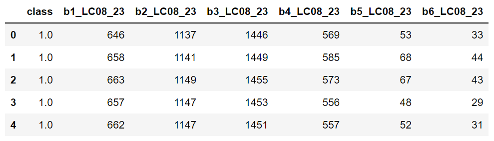
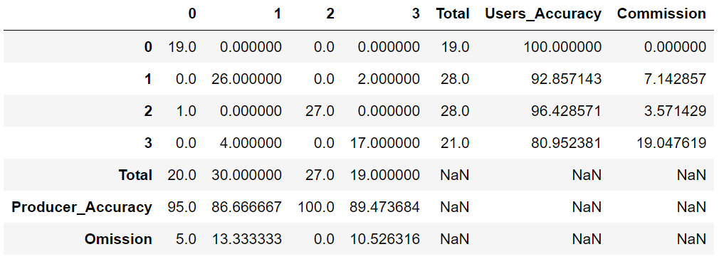
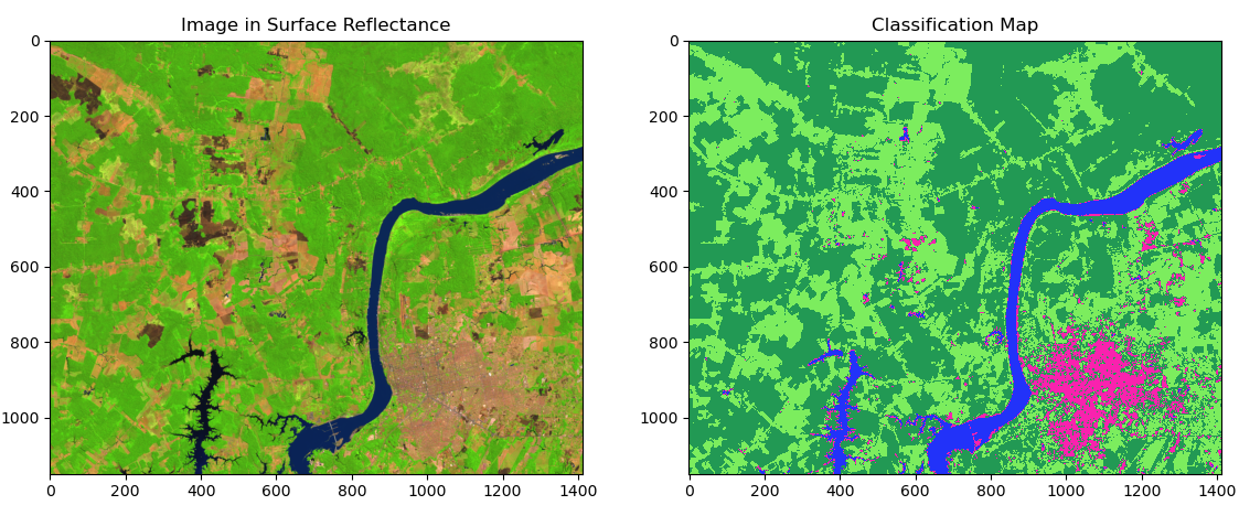
In this example, in a small region of southern Brazil, optical imagery from Landsat-8 OLI (Operational Land Imager) will be used to classify land cover using the machine learning algorithm Random Forest (RF) (Breiman, 2001). Four types of land cover will be mapped, i.e., agriculture, forest, bare soil and water. The input data needed is the satellite image and the spectral signatures collected. The output as a dictionary will provide: i) confusion matrix, ii) overall accuracy, iii) kappa index and iv) a classes map.

01. Optical image to be used

Landsat-8 OLI (Operational Land Imager) will be used to obtain in order to classify using Random Forest (RF). This image, which is in surface reflectance with bands:

• Blue -> B2
• Green -> B3
• Red -> B4
• Nir -> B5
• Swir1 -> B6
• Swir2 -> B7

The image and signatures to be used can be downloaded here:

02. Libraries to be used in this example

import rasterio
import numpy as np
from scikeo.mla import MLA
import matplotlib.pyplot as plt
from dbfread import DBF
import matplotlib as mpl
import pandas as pd

03. Image and endmembers

We will upload a satellite image as a .tif and endmembers as a .dbf.

path_raster = r"C:\data\ml\LC08_232066_20190727_SR.tif"
img = rasterio.open(path_raster)

path_endm = r"C:\data\ml\endmembers.dbf"
endm = DBF(path_endm)

# endmembers
df = pd.DataFrame(iter(endm))
df.head()

04. Classifying with Random Forest

An instance of mla():

inst = MLA(image = img, endmembers = endm)

Applying with 70% of data to train:

rf_class = inst.SVM(training_split = 0.7)

5.0 Results

Dictionary of results

rf_class.keys()

Overall accuracy

rf_class.get('Overall_Accuracy')

Kappa index

rf_class.get('Kappa_Index')

Confusion matrix or error matrix

rf_class.get('Confusion_Matrix')

06. Preparing the image before plotting

# Let's define the color palette
palette = mpl.colors.ListedColormap(["#2232F9","#F922AE","#229954","#7CED5E"])

Applying the plotRGB() algorithm is easy:

# Let´s plot
fig, axes = plt.subplots(nrows = 1, ncols = 2, figsize = (15, 9))

# satellite image
plotRGB(img, title = 'Image in Surface Reflectance', ax = axes[0])

# class results
axes[1].imshow(svm_class.get('Classification_Map'), cmap = palette)
axes[1].set_title("Classification map")
axes[1].grid(False)

Example 02: Calibration methods for supervised classification

Given a large number of machine learning algorithms, it is necessary to select the one with the best performance in the classification, i.e., the algorithm in which the training and testing data used converge the learning iteratively to a solution that appears to be satisfactory (Tarazona et al., 2021). To deal with this, users can apply the calibration methods Leave One Out Cross-Validation (LOOCV), Cross-Validation (CV) and Monte Carlo Cross-Validation (MCCV) in order to calibrate a supervised classification with different algorithms. The input data needed are the spectral signatures collected as a .dbf or .csv. The output will provide a graph with the errors of each classifier obtained.

01. Endmembers as a .dbf

path_endm = "\data\ex_O2\\endmembers\endmembers.dbf"
endm = DBF(path_endm)

02. An instance of calmla()

inst = calmla(endmembers = endm)

03. Applying the splitData() method

data = inst.splitData()

Calibrating with Monte Carlo Cross-Validation Calibration (MCCV)

Parameters:

• split_data: An instance obtaind with splitData().
• models: Support Vector Machine (svm), Decision Tree (dt), Random Forest (rf) and Naive Bayes (nb).
• n_iter: Number of iterations.

04. Running MCCV

error_mccv = inst.MCCV(split_data = data, models = ('svm', 'dt', 'rf', 'nb'), 
                       n_iter = 10)

Calibration results:

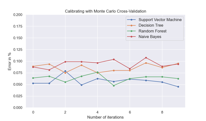
With this result it can be observed that SVM and RF obtained a higher overall accuracy (less error). Therefore, you can use these algorithms to classify a satellite image.

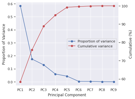
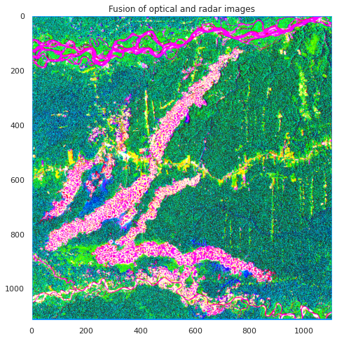
Example 03: Imagery Fusion - optical/radar

This is an area where scikit-eo provides a novel approach to merge different types of satellite imagery. We are in a case where, after combining different variables into a single output, we want to know the contributions of the different original variables in the data fusion. The fusion of radar and optical images, despite of its well-know use, to improve land cover mapping, currently has no tools that help researchers to integrate or combine those resources. In this third example, users can apply imagery fusion with different observation geometries and different ranges of the electromagnetic spectrum (Tarazona et al., 2021). The input data needed are the optical satellite image and the radar satellite image, for instance.

In scikit-eo we developed the function fusionrs() which provides us with a dictionary with the following image fusion interpretation features:

• Fused_images: The fusion of both images into a 3-dimensional array (rows, cols, bands).
• Variance: The variance obtained.
• Proportion_of_variance: The proportion of the obtained variance.
• Cumulative_variance: The cumulative variance.
• Correlation: Correlation of the original bands with the principal components.
• Contributions_in_%: The contributions of each optical and radar band in the fusion.

01. Loagind dataset

Loading a radar and optical imagery with a total of 9 bands. Optical imagery has 6 bands Blue, Green, Red, NIR, SWIR1 and SWIR2, while radar imagery has 3 bandas VV, VH and VV/VH.

path_optical = "data/ex_03/LC08_003069_20180906.tif"
optical = rasterio.open(path_optical)

path_radar = "data/ex_03/S1_2018_VV_VH.tif"
radar = rasterio.open(path_radar)

02. Applying the fusionrs:

fusion = fusionrs(optical = optical, radar = radar)

03. Dictionary of results:

fusion.keys()

04. Proportion of variance:

prop_var = fusion.get('Proportion_of_variance')

05. Cumulative variance (%):

cum_var = fusion.get('Cumulative_variance')*100

06. Showing the proportion of variance and cumulative:

x_labels = ['PC{}'.format(i+1) for i in range(len(prop_var))]

fig, axes = plt.subplots(figsize = (6,5))
ln1 = axes.plot(x_labels, prop_var, marker ='o', markersize = 6,  
                label = 'Proportion of variance')

axes2 = axes.twinx()
ln2 = axes2.plot(x_labels, cum_var, marker = 'o', color = 'r', 
                 label = "Cumulative variance")

ln = ln1 + ln2
labs = [l.get_label() for l in ln]

axes.legend(ln, labs, loc = 'center right')
axes.set_xlabel("Principal Component")
axes.set_ylabel("Proportion of Variance")
axes2.set_ylabel("Cumulative (%)")
axes2.grid(False)
plt.show()

07. Contributions of each variable in %:

fusion.get('Contributions_in_%')

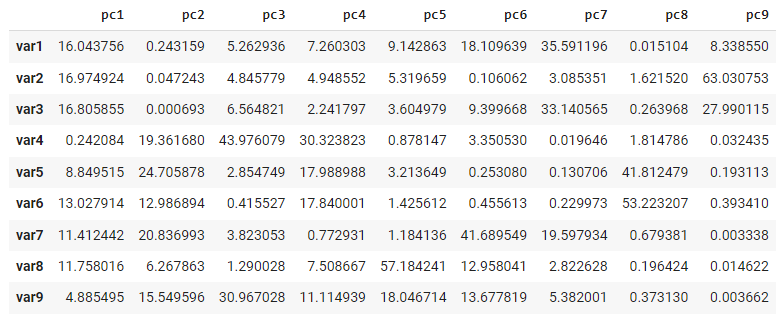
Here, var1, var2, ... var12 refer to Blue, Green, ... VV/VH bands respectively. It can be observed that var2 (Green) has a higher contribution percentage 16.9% than other variables. With respect to radar polarizaciones, we can note that var8 (VH polarization) has a higher contribution 11.8% than other radar bands.

08. Preparing the image:

arr = fusion.get('Fused_images')

## Let´s plot
fig, axes = plt.subplots(figsize = (8, 8))
plotRGB(arr, bands = [1,2,3], title = 'Fusion of optical and radar images')
plt.show()

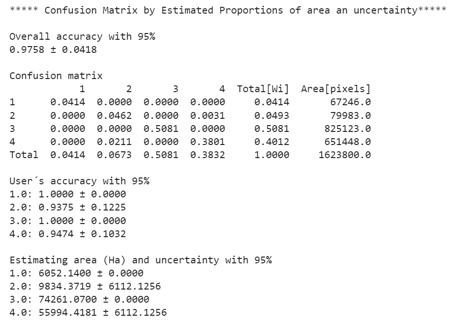
Example 04: Confusion matrix by estimated proportions of area with a confidence interval at 95%

In this final example, after obtaining the predicted class map, we are in a case where we want to know the uncertainties of each class. The assessing accuracy and area estimate will be obtained following guidance proposed by (Olofsson et al., 2014). All that users need are the confusion matrix and a previously obtained predicted class map.

confintervalML requires the following parameters:

• matrix: confusion matrix or error matrix in numpy.ndarray.
• image_pred: a 2-dimensional array (rows, cols). This array should be the classified image with predicted classes.
• pixel_size: Pixel size of the classified image. Set by default as 10 meters. In this example is 30 meters (Landsat).
• conf: Confidence interval. By default is 95% (1.96).
• nodata: No data must be specified as 0, NaN or any other value. Keep in mind with this parameter.

#### 01. Load raster data
path_raster = r"\data\ex_O4\ml\predicted_map.tif"
img = rasterio.open(path_optical).read(1)

#### 02. Load confusion matrix as .csv
path_cm = r"\data\ex_O4\ml\confusion_matrix.csv"
values = pd.read_csv(path_radar)

#### 03. Applying the confintervalML:
confintervalML(matrix = values, image_pred = img, pixel_size = 30, conf = 1.96, 
               nodata = -9999)

Results:

---

Last update: 2023-08-02